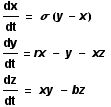
 The Lorenz equations are a set of three coupled non-linear ordinary differential equations (ODE). They make up a simplified system describing the two-dimensional flow of a fluid. As can be seen, the derivative of all three variables is given with respect to t, and as a function involving one or both of the other variables (thus they are said to be coupled). The usual values taken by the parameters are as follows:
sigma = 10, r = 28, and b = 8/3.
As time is incremented then, the calculated values of x, y, z change as shown in the timeseries plot below. x = red, y = green, z = blue.
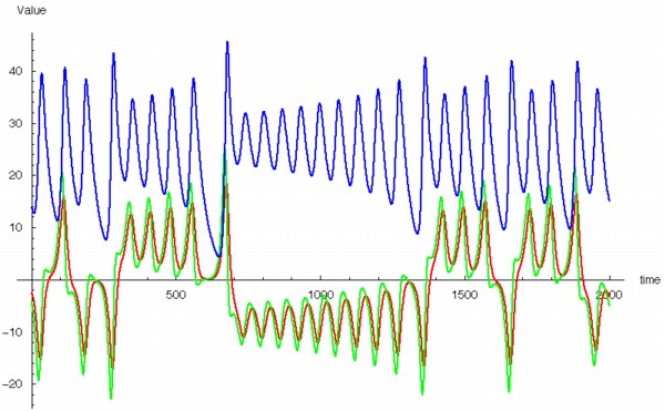
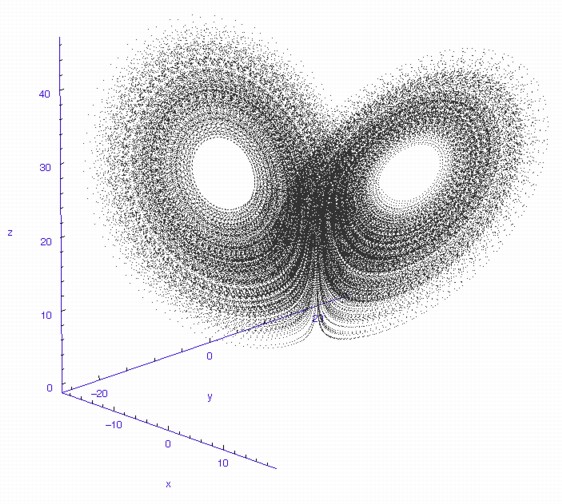
 The fluctuations are seemingly utterly random. More structure can be seen, however, if the same timeseries is plotted as a sequence of co-ordinates describing a trajectory through 3-space. As shown to the right, the surface resembles a twisted bow-tie. It is known as the Lorenz strange attractor, and no equilibrium (dynamic or static) is ever reached – it does not form limit cycles or achieve a steady state. Thus, no trajectory ever coincides with any other. Instead, it is an example of deterministic chaos, one of the first realised by mathematicians.
One of the properties of a chaotic system is that it is sensitive to initial conditions. This means that no matter how close two different initial states are (i.e. even down to the 20th decimal place) their trajectories will soon diverge. This is popularly referred to as the “Butterfly Effect”, whereby small changes in the initial state can lead to rapid and dramatic differences in the outcome. The metaphor is that a butterfly flapping its wings in Brazil could result in a tornado in Texas.
The Lorenz equations cannot be solved analytically by integration. Instead, a numerical approximation technique must be used. The 4th order Runge-Kutta (RK) method employed here takes a weighted average of four estimates of the derivative at a point in order to calculate the new position after a time increment. The lower-order error terms cancel out, making RK very robust despite its simplicity.
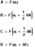 To generate all of these images and animations, a Mathematica programme was written to perform the RK numerical analysis of the Lorenz equations. For the initial state, an arbitrary point in 3-space, ut , is chosen, and then four derivatives calculated (A, B, C and D) using a time increment of h. In each case, F is the three-dimensional vector function composed of the Lorenz differential equations given above. These derivatives are weighted and combined to give the approximation for the next point, ut+h .
![]()
The three components of this point are appended to a storage list, and then the whole calculation reiterated a large number of times. For the high resolution image above, 100,000 co-ordinates were calculated and plotted, expending almost an hour of computer runtime. For the animation below, only 10,000 points were used.
 Once calculated, all of the points in this data list are plotted in order to visualise the Lorenz attractor. This draw command was placed in a programme loop, with the x, y, and z co-ordiantes of the viewing-point for the projection incremented each time to generate a string of images. These were then converted into an animated .gif to create the rotating attractor shown to the left.
The animation of the trajectory through time (shown at the top) was created by calculating just 1,000 co-ordinates, starting with a point known to be near the transition region between the two lobes. Only a subset of these points were plotted each time in the draw loop, beginning with the first 5, then the first 10, first 15, 20, 25, and so on.
2 replies on “Runge-Kutta and the Lorenz Attractor”
Your explanation was very helpful. Thanks.
More than welcome!